
Data Acquisition and Sensor Calibration | ACE-Lab Operate · Control Engineering
Data Acquisition and Sensor Calibration
Explore how measurement signals are acquired by a microcontroller and converted from raw electrical or digital information into meaningful engineering quantities using conversion, scaling and basic calibration.
Contents
Key Learning Outcomes
By the end of this section, you should be able to:
01 Identify the role of the measurement device and microcontroller input interface within a control-system block diagram.
02 Distinguish between digital-state measurements, digitally encoded measurements and analogue measurements.
03 Explain ADC resolution and quantisation, and convert a raw 10-bit ADC reading into a corresponding input voltage.
04 Apply basic scaling and calibration to convert raw sensor data into a meaningful engineering quantity.
Measurement in a Control System
A control system is commonly represented using a block diagram consisting of a control algorithm, system (plant/process), measurement device and feedback. The Arduino Uno R3 provides the physical hardware needed to acquire measurement signals and process them in software.
Here, attention is directed towards the measurement device and the path used to convert a sensed physical quantity into information that can be used by the control algorithm. Examples include converting an ultrasonic echo time into distance, or converting an analogue sensor voltage into temperature, light level or position.
Figure 5: Block Diagram Form for a Control System As shown in Figure 5, the measurement device provides the information returned through the feedback path. Before that information can be used, the microcontroller must acquire the incoming signal and convert it into a numerical representation.
Figure 6: Algorithm and Measurement Device are Now Considered In Figure 6, the Arduino Uno receives the signal produced by the measurement device. These inputs are acquired in two primary ways:
- Digital input pins for discrete logic states or digitally encoded timing information.
- Analogue input pins for continuously varying voltages that are converted into numerical values by the analogue-to-digital converter (ADC).
At this stage, the summing junction used to generate the error, e, is not considered. The focus is the measurement path itself: acquiring the signal, interpreting it and producing a usable measurement.
From Sensor Signal to Engineering Quantity
A raw signal at a microcontroller pin does not automatically provide a meaningful engineering measurement. Several steps may be required before the signal can be interpreted as a physical quantity such as distance, temperature, light level or position.
Physical quantityDistance, light, temperature, position, etc.Sensor / transducerConverts the physical quantity into an electrical or timed signal.AcquisitionDigital input timing or analogue sampling captures the signal.ConversionTiming, ADC conversion or decoding produces a raw numerical value.Scaling / calibrationConverts the raw value into meaningful engineering units.Measurement is more than reading a pin. A reliable measurement chain must preserve the relationship between the physical quantity and the number used by the control algorithm.Digital Inputs for Measurement
A digital sensor communicates with the microcontroller using either discrete logic levels or digitally encoded signals. Although both use digital pins, the information represented by the signal is different.
Discrete logic measurement
The input is interpreted directly as HIGH or LOW. The state can represent whether a condition is satisfied, such as a switch being pressed or an object being detected.
Digitally encoded measurement
The physical quantity is represented through timing, pulse width or a structured digital data stream. Software must interpret the signal before a numerical measurement is obtained.
The HC-SR04 ultrasonic sensor is an example of a digitally timed measurement. A short trigger pulse starts a measurement and the duration of the returned echo pulse represents the acoustic round-trip travel time. The distance is therefore obtained from:
(2)In Equation (2), d is the measured distance, c is the assumed speed of sound and techo is the measured echo-pulse duration. The division by two accounts for the outward and return journey of the sound wave.
ACE-Box (Base + Sense): Ultrasonic Sensor Exercise
The ultrasonic exercise moves measurement from a block-diagram concept into a real embedded workflow. You will generate a trigger signal, measure the returning echo timing and convert that timing into a distance measurement in Simulink.
Why this exercise matters: it demonstrates that a digital input does not always represent a simple ON/OFF state. A measurement can be encoded in the timing of a digital signal, so reliable acquisition depends on both correct hardware configuration and correct interpretation in software.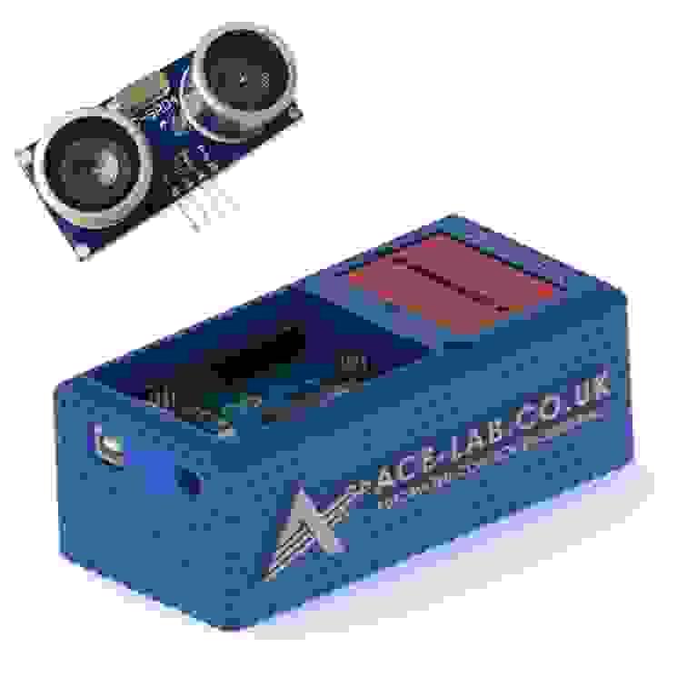 Base + SenseEstimated time: 1 hour
Ultrasonic Sensor (Distance)
Measure distance with an HC-SR04 ultrasonic sensor and use simple logic to improve the reliability of the reported measurement.
Open ExerciseReflective Questions
Click a question block to reveal the suggested answer. The answer will slide out directly below the question; click the block again to close it.
The trigger initiates the ultrasonic burst and the echo-pulse duration represents the round-trip travel time of the sound. Distance is calculated using Equation (2), so the measured time is multiplied by the assumed speed of sound and divided by two. This assumes that the sound travels to the target and back along the expected path and that the value used for the speed of sound is sufficiently accurate for the operating conditions.Ultrasonic measurements can be affected by weak or missing echoes, angled or absorbent surfaces, objects outside the useful range, reflections from other surfaces and occasional invalid timing values. Last Good Value logic rejects an invalid result and temporarily retains the most recent valid measurement. This improves continuity, although the retained value should not be treated as a new measurement if the real distance is changing rapidly.The sample time must allow the trigger–echo measurement sequence to complete and must provide an appropriate update rate for the application. Sampling too slowly reduces the rate at which distance changes can be observed, while triggering too quickly can create overlapping or invalid measurements. The Simulink pin assignments must also match the physical trigger and echo connections; an incorrect assignment prevents the timing information from being generated or acquired correctly.Analogue Inputs and the ADC
The Arduino Uno R3 acquires analogue measurements using its built-in 10-bit analogue-to-digital converter (ADC). The voltage arriving at an analogue input is continuous, but the ADC converts that voltage into a discrete numerical code that can be processed in software.
For a 10-bit ADC, the number of available quantisation levels is 210 = 1024, producing integer output codes from 0 to 1023. The smallest voltage step represented by one ADC level is:
(3)In Equation (3), Vref is the ADC reference voltage and n is the ADC resolution in bits. For a standard 5 V reference and a 10-bit ADC:
(4)Equation (4) means that one ADC count corresponds to approximately 4.88 mV when a 5 V reference is used. A change smaller than one quantisation step cannot be represented as a separate ADC code.
The mapping of a continuous input voltage to one of 1024 discrete levels is called quantisation. Quantisation therefore places a fundamental limit on measurement resolution: the ADC can only report one of the available codes, not every possible input voltage.
Resolution is not the same as accuracy. A 10-bit ADC can represent 1024 levels, but the accuracy of the final engineering measurement also depends on the sensor, reference voltage, electrical noise, scaling and calibration.Scaling and Sensor Calibration
Reading an ADC code is only the beginning of the measurement process. The raw value must usually be converted into the units required by the application. Scaling changes the numerical range, while calibration uses known reference values to improve the relationship between the measured signal and the actual physical quantity.
Scaling
Applies a known mathematical conversion, for example mapping an ADC range of 0–1023 to 0–5 V or mapping a slider position to a required command range.
Calibration
Compares the sensor output with one or more known reference values so that gain and offset errors, and where necessary nonlinear behaviour, can be accounted for.
For a measurement that can be approximated by a linear relationship, a simple calibrated engineering quantity, x, can be written as:
(5)In Equation (5), N is the raw measurement value, m is a scale factor and b is an offset. The values of m and b may come from a known sensor relationship or may be determined experimentally using reference measurements.
This distinction becomes important when comparing different sensors. A slide potentiometer often provides an approximately linear relationship between position and voltage, whereas an LDR is typically nonlinear and is also influenced by the surrounding circuit. The same ADC can acquire both signals, but the conversion from raw ADC code to the desired engineering quantity may be different.
ACE-Box (Base + Sense): Slide Potentiometer and LDR Exercises
These two exercises use the same analogue input hardware but represent two different measurement situations. The slide potentiometer provides a deliberate, user-controlled change in position, while the LDR responds to changes in the surrounding light level.
Why these exercises matter: together they show that acquiring an analogue voltage is only one part of measurement. You must also consider ADC resolution, the useful signal range, scaling and the physical relationship between the sensor output and the quantity you want to represent.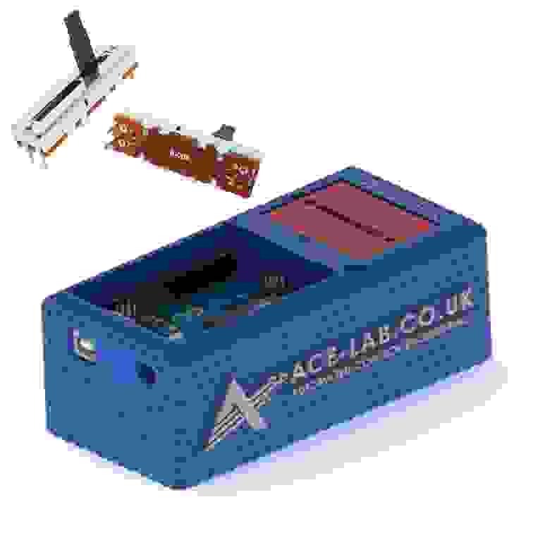 Base + SenseEstimated time: 0.5 hour
Slide Potentiometer
Read the potentiometer through the ADC, inspect the raw 10-bit value and scale the measurement to a useful numerical range in Simulink.
Open Exercise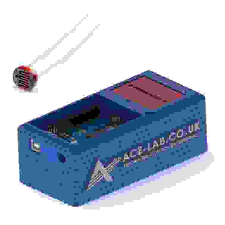 Base + SenseEstimated time: 0.5 hour
LDR (Light Dependent Resistor)
Measure a light-dependent analogue voltage using an LDR circuit and consider how the acquired ADC value can be scaled or calibrated for monitoring and control.
Open ExerciseReflective Questions
Click a question block to reveal the suggested answer. The answer will slide out directly below the question; click the block again to close it.
The ADC produces values from 0 to 1023, while an 8-bit PWM command typically uses 0 to 255. A suitable scale factor maps the full input range to the full output range. If the factor is too large, the PWM command reaches its maximum before the potentiometer reaches the end of its travel, causing early saturation. If it is too small, the available PWM range is not fully used, reducing the useful brightness range and effective command resolution.Both exercises produce a changing analogue voltage that is sampled by the same ADC, so the acquisition process is similar. The potentiometer is intentionally moved by the user and is usually close to a linear position-to-voltage relationship. The LDR responds to the environment, may change less predictably and has a nonlinear resistance-to-light relationship. The LDR model may therefore require different scaling, calibration and possibly filtering compared with the potentiometer.The ADC conversion only estimates the voltage presented at the input pin. The final engineering value also depends on the sensor transfer relationship, component tolerances, reference-voltage accuracy, offset, gain error, noise and any nonlinearity. Calibration links the acquired electrical value to known physical reference values so that the reported engineering measurement better represents the real quantity.Concluding Remarks
This section has introduced the measurement path used to convert sensor behaviour into information that can be processed by a microcontroller. Digital inputs may represent either simple logic states or measurements encoded through signal timing, while analogue inputs rely on the ADC to convert continuous voltage into discrete numerical levels.
Most importantly, a raw digital or ADC value is not automatically a meaningful engineering measurement. Conversion, scaling and calibration provide the link between the electrical signal and the physical quantity being measured. The ACE-Lab exercises reinforce this progression by moving from ultrasonic timing to analogue position and light measurements, providing the measurement foundation required before those signals are used within a complete feedback-control system.