


Quanser QCar 2 | Longitudinal Speed Control Quanser QCar 2Longitudinal Speed Control
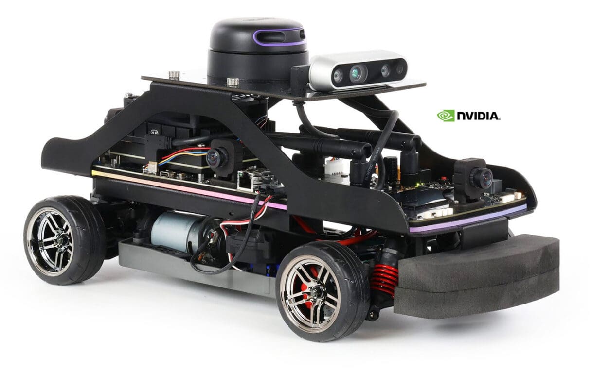
Explore longitudinal speed control through a structured control engineering journey, progressing from understanding the QCar 2 speed-control problem and its requirements, through ACE-CORE and ACE-Lab activities that develop the underlying knowledge, to model-based control-system design.
 C
CComprehend
What are we trying to control?Develop a basic understanding of the QCar 2 longitudinal speed-control problem, including the desired speed, measured speed, feedback and error, the basic closed-loop arrangement, the vehicle speed response and the requirements used to describe satisfactory speed-control performance.
Learn, then apply
Complete each ACE-CORE topic, then apply the idea directly to the Quanser QCar 2 longitudinal speed-control problem.
Consider the QCar 2 longitudinal speed-control problem. The aim is for the vehicle's actual speed to follow a desired speed.
Part AIdentify the speed-control quantities
- What physical quantity is being controlled on the QCar 2?
- What quantity represents how fast we want the QCar 2 to travel?
- What quantity tells us how fast the QCar 2 is actually travelling?
- Controlled quantity: longitudinal speed
- Desired quantity: desired longitudinal speed
- Measured quantity: actual longitudinal speed
Part BDescribe the speed-control objective
- In one sentence, describe what the QCar 2 longitudinal speed-control system should achieve.
- Why might applying the same drive command not always result in exactly the same vehicle speed?
The longitudinal speed-control system should make the actual QCar 2 speed follow the desired QCar 2 speed.
A drive command alone does not guarantee a particular speed because the physical vehicle can respond differently under different operating conditions.
Assume the desired QCar 2 longitudinal speed is 0.80 m/s. The measured speed is fed back and compared with this desired value.
Part ACalculate the longitudinal speed error
Desired QCar 2 speed (m/s) Measured QCar 2 speed (m/s) Speed error (m/s) 0.80 0.30 ? 0.80 0.70 ? 0.80 0.80 ? 0.80 0.90 ? Using speed error = desired speed − measured speed :
- 0.80 − 0.30 = +0.50 m/s
- 0.80 − 0.70 = +0.10 m/s
- 0.80 − 0.80 = 0.00 m/s
- 0.80 − 0.90 = −0.10 m/s
Part BInterpret the speed error
- What does a positive QCar 2 speed error mean?
- What does zero speed error mean?
- What does a negative QCar 2 speed error mean?
- Positive speed error means the QCar 2 is travelling slower than the desired speed.
- Zero speed error means the measured speed is equal to the desired speed.
- Negative speed error means the QCar 2 is travelling faster than the desired speed.
Part CWhy is speed feedback useful?
Why is feeding the measured QCar 2 longitudinal speed back into the control system useful?
Speed feedback allows the actual QCar 2 speed to be compared with the desired QCar 2 speed. This comparison produces the speed error and shows whether the vehicle is travelling too slowly, at the desired speed, or too quickly.
Now map the basic feedback-control structure onto the QCar 2 longitudinal speed-control problem.
Part AIdentify the QCar 2 speed-control elements
For the QCar 2 longitudinal speed-control loop, identify:
- The desired input.
- The measured output.
- The error signal.
- The generic controller block.
- The physical system being controlled.
- The feedback signal.
- Desired input: desired QCar 2 longitudinal speed
- Measured output: actual QCar 2 longitudinal speed
- Error signal: desired speed minus measured speed
- Controller: a generic speed-control block
- Physical system: the QCar 2 drive system and longitudinal motion
- Feedback signal: measured longitudinal speed
Part BConnect the QCar 2 speed-control loop
Sketch the basic closed-loop arrangement for QCar 2 longitudinal speed control using the elements identified in Part A.
At this stage, do not choose a specific controller type.
The basic speed-control structure should follow:
Desired QCar 2 speed → speed comparison → speed error → controller → QCar 2 drive system → measured QCar 2 speed
The measured longitudinal speed is then fed back to the speed comparison point.
Imagine that the desired QCar 2 speed changes from 0 m/s to 0.80 m/s. The measured longitudinal speed rises towards the target, briefly exceeds it and then settles close to 0.80 m/s.
Part ADescribe the QCar 2 speed response
- What does rise time describe for the QCar 2 speed response?
- What does overshoot describe?
- What does settling time describe?
- What does steady-state error describe?
- Rise time: how quickly the QCar 2 speed rises towards the desired speed.
- Overshoot: how far the QCar 2 speed exceeds the desired speed.
- Settling time: how long the QCar 2 speed takes to remain sufficiently close to the desired speed.
- Steady-state error: the remaining difference between desired and measured QCar 2 speed after the response has settled.
Part BRecognise desirable speed-control behaviour
For the QCar 2 longitudinal speed response, would you generally prefer the following to be larger or smaller?
- Rise time
- Overshoot
- Settling time
- Steady-state speed error
In general, a well-behaved QCar 2 speed response would aim for:
- shorter rise time
- less speed overshoot
- shorter settling time
- smaller steady-state speed error
Consider the desired behaviour for the QCar 2: the vehicle should reach the requested longitudinal speed quickly, avoid excessive speed overshoot and then maintain the requested speed accurately.
Part AMatch QCar 2 speed behaviour to a measure
- Which measure describes how quickly the QCar 2 reaches the requested speed?
- Which measure describes how far the QCar 2 speed exceeds the requested speed?
- Which measure describes the remaining difference between the requested and measured speed once the response has settled?
- Time taken to reach the requested speed: rise time
- Speed exceeding the requested value: overshoot
- Remaining speed difference after settling: steady-state error
Part BMake the QCar 2 speed requirements measurable
Rewrite each statement so that the QCar 2 longitudinal speed response could later be measured and tested.
- "The QCar 2 should reach the requested speed quickly."
- "The QCar 2 should not exceed the requested speed by too much."
- "The QCar 2 should maintain the requested speed accurately."
Example measurable forms are:
- QCar 2 speed rise time should be less than a specified time.
- QCar 2 speed overshoot should be below a specified percentage.
- QCar 2 steady-state speed error should remain within a specified speed tolerance.
The important idea at this stage is to turn the desired speed behaviour into something that can later be measured and tested.
OOperate
What practical understanding do we need?Use ACE-CORE together with ACE-Lab to develop the practical understanding needed for longitudinal speed control, exploring how sensing, actuation and embedded control are implemented.
Learn, then practise
Use ACE-CORE to establish the embedded-control concept, then use ACE-Lab to investigate it physically. The Quanser QCar 2 provides the application context, but the practical development in Operate is carried out using ACE-Lab.
Before working with individual inputs and outputs, identify the role played by the microcontroller within ACE-Lab.
Part AIdentify the embedded-control functions
- What is the role of the microcontroller within ACE-Lab?
- What types of information can enter the microcontroller as inputs?
- What types of signals can the microcontroller generate as outputs?
- Why is a microcontroller useful when a control algorithm must operate repeatedly in real time?
The microcontroller provides the embedded computational platform for the control system. It can acquire input signals, execute the programmed algorithm and generate output commands.
Inputs can include digital or analogue measurements from switches and sensors. Outputs can include digital states and PWM commands used to drive devices or, through suitable interface hardware, actuators.
ACE-Lab platform: use the Base + Sense and Actuate hardware to identify where measurement signals enter the embedded controller and where control commands leave it.Use a simple output device before moving to a motor. This isolates the key embedded-control ideas of digital output, PWM and repeated execution without introducing actuator dynamics yet.
Part ADigital output
Complete the LED digital-output practical and identify the relationship between the logical output command and the physical LED state.
- What happens when the digital output is switched between LOW and HIGH?
- Why is this described as a discrete or two-state output?
Part BPulse-width modulation
Replace the simple on/off command with PWM and investigate how changing duty cycle changes the average output delivered to the load.
- Increase and decrease PWM duty cycle and observe the LED response.
- Explain why PWM is useful when a digital microcontroller must vary the effective output applied to a physical device.
- Relate the model sample time to how often the output command is recalculated and updated.
P1 · LED (Digital) Establish basic digital-output operation using a simple two-state physical output.P2 · LED (PWM) Introduce PWM duty cycle before the same principle is later used to command an actuator.Why this is an extension: O04 explains how polarity and PWM control the motor. Here, combine those ideas into a single command format that will later be much easier for a feedback controller to generate.Extension taskMap a signed command to direction and PWM
Define a normalised motor command u in the range -1 ≤ u ≤ +1.
PWM = 255|u|
sign of u → motor direction- Complete the direction and PWM command for u = -1.0, -0.4, 0, +0.4 and +1.0.
- Explain why u = 0 should produce a zero motor command.
- Explain why this signed representation is useful when a controller later calculates the actuator command automatically.
u Direction PWM magnitude -1.0 ? ? -0.4 ? ? 0 ? ? +0.4 ? ? +1.0 ? ? - -1.0 → reverse, PWM 255
- -0.4 → reverse, PWM ≈ 102
- 0 → stop, PWM 0
- +0.4 → forward, PWM ≈ 102
- +1.0 → forward, PWM 255
A signed command is useful because the controller can produce one value whose sign determines direction and whose magnitude determines drive level.
Bridge towards the application: ACE-Lab gives a rotational speed measurement in RPM, whereas vehicle longitudinal speed is normally expressed in m/s. Converting between the two starts connecting the motor-level measurement to the vehicle-level quantity of interest.Extension taskRPM → m/s
If the measured rotational speed is n RPM and the effective wheel or roller radius is r metres:
v = 2πr × n / 60
where v is linear speed in m/sFor this exercise, assume an effective radius of r = 0.030 m and direct drive.
Rotational speed Linear speed 30 RPM ? 60 RPM ? 90 RPM ? - Calculate the corresponding linear speed for 30, 60 and 90 RPM.
- Plot or display both RPM and m/s from the same measured motor-speed signal.
- Explain why the conversion factor depends on wheel radius.
- 30 RPM → approximately 0.094 m/s
- 60 RPM → approximately 0.188 m/s
- 90 RPM → approximately 0.283 m/s
If the measured RPM is taken before a gearbox or transmission, first convert motor RPM to wheel RPM using the relevant transmission ratio.
The 0.030 m radius is an illustrative value for the extension exercise, not a stated QCar 2 wheel dimension.
Bridge towards longitudinal speed control: the PI controller operates on the motor-speed variable, but the application requirement may be written in m/s. Add a conversion layer so a linear-speed reference can be turned into the RPM reference required by the motor controller.Extension taskm/s → RPM → PI control → m/s
Rearranging the O05 conversion gives:
n = 60v / (2πr)
where n is RPM and v is linear speed in m/sContinue using the illustrative radius r = 0.030 m.
- Calculate the RPM reference corresponding to a desired linear speed of 0.20 m/s.
- Feed this RPM value into the PI speed-control system as the reference.
- Convert the measured RPM back into m/s and display desired and measured linear speed on the same scope.
- Assess rise time, overshoot and steady-state error using m/s rather than RPM.
For v = 0.20 m/s and r = 0.030 m:
n = 60 × 0.20 / (2π × 0.030) ≈ 63.7 RPM
The PI controller can therefore still operate on RPM internally, while the user sets and observes the higher-level speed variable in m/s.
This extension deliberately creates a conceptual bridge from ACE-Lab motor speed control to vehicle longitudinal speed control, without requiring the QCar 2 hardware during Operate.
RRefine
How can control performance be improved?Continue using ACE-CORE and ACE-Lab to explore how an operating control system can be assessed, adjusted and retested to improve its performance.
EEngineer
How can model-based design improve performance and reduce development time?Apply a model-based design approach to develop the QCar 2 longitudinal speed-control system, using modelling, simulation and controller design to improve speed-control performance, reduce physical testing and accelerate implementation.